
2020-03-05
Mapping Robot for highly accurate Indoor Datasets
Parts of this project are available on GitHub.
The work presented here was part of a semester project at the TU Berlin’s Daimler Center for automotive IT Innovations.
The goal of this semester project was to create colored point clouds of indoor environments. To achieve this, my group partner and I were given a mobile robot with a 360° camera and two laser scanners (lidars) with the task of writing a software that merges point cloud data with RGB images to generated a colored point cloud.
This article describes the progress we made during the semester and the architecture and capabilities of the final implementation.
1 System Overview
The robot was remote controlled and driven through a building, while it was recording lidar scans and camera images. After the run, the collected data was to be merged into a colored point cloud (point positions from lidars and colors from camera) that represented a 3D map of the building the robot was driving through.
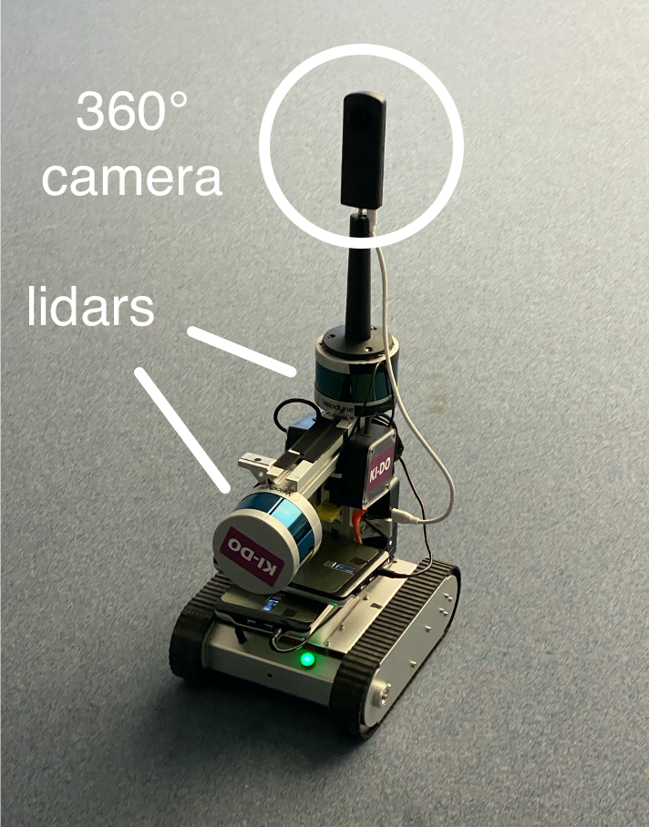
It was equipped with an Intel Nuc running the Robot Operating System (ROS) and had two Velodyne Puck lidars attached to it. Data was recorded to a rosbag file using the Velodyne ros driver node. It also had wheel encoders mounted to collect odometry information.
The camera which was mounted on top of the robot is a Ricoh Theta Z1 360° camera which unfortunately stops every 4K recording automatically after just five minutes. This information was hidden somewhere in the dataset and of course had a negative impact on the data collection runs. It also does not have a ros driver or a reliable way of streaming 4K video to the Nuc.
At the end of each run, we had a video file from the camera and a rosbag containing odometry information and laser scans.
As described so far, the robot was given to us at the beginning of the project phase and groups in previous years had worked on building the robot and established the remote control.
The recorded data was then used as an input to the processing pipeline above which created a colored 3D pointcloud from the data after the run. The processing was not done on the robot in real time, as the robot’s task did not include autonomous exploration and map building at runtime was not required (in addition to the nuc being to weak and some other limiting factors like the consumer grade camera).
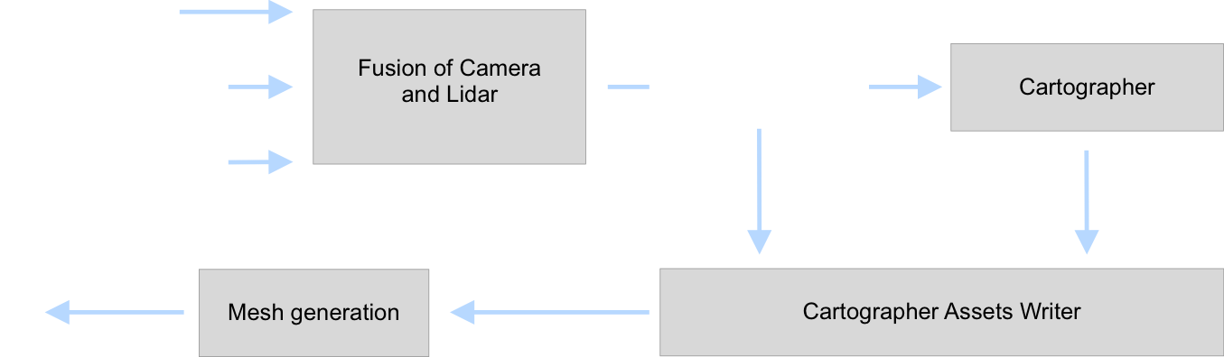
The processing pipeline is summarized in the figure above. A first step was coloring the collected scan messages in the rosbag with the colors obtained from the camera’s video. This could be done before building a pointcloud, because the transformation (position and rotation difference) between the laser scanners and the camera never changed.
From there on, processing continued with a single rosbag file. We used Google’s cartographer to as a SLAM algorithm. What a SLAM algorithm is and what it does is explained in the next section.
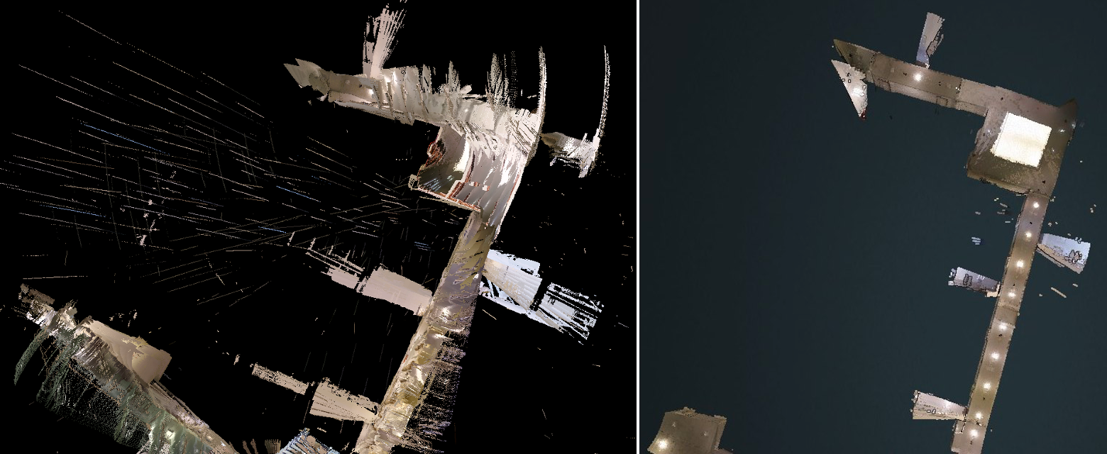
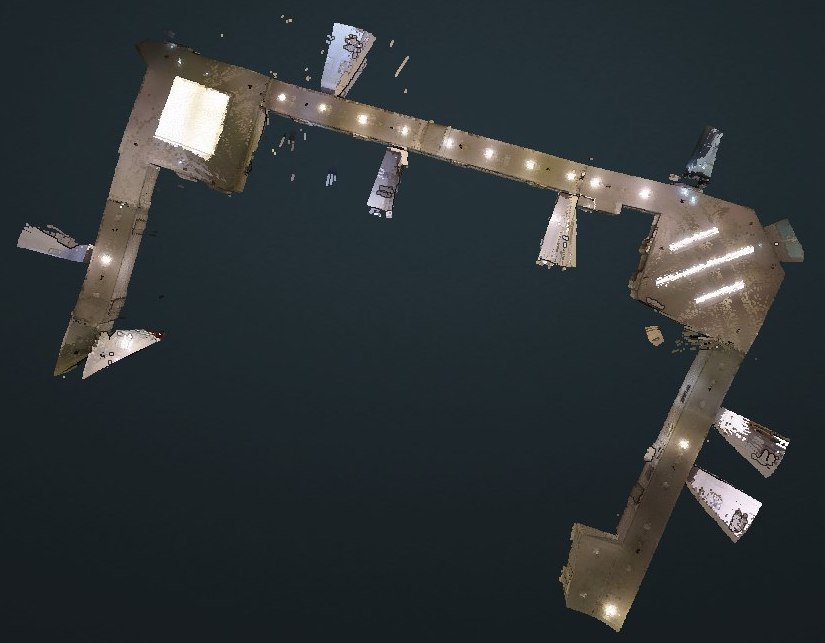
After the cartographer returned a point cloud, we generated a mesh from the point cloud which was a digital copy of the environment the robot was traveling through.
2 Cartographer
We used Cartographer version 1.0.0 for our fork. In early 2021, version 2.0.0 was released.
Cartographer is a SLAM (simultaneous localization and mapping) algorithm developed by Google. As the name implies, it consumes data like laser scans from a moving robot and creates a map of the environment through which the robot is traveling while also locating the robot in that map. Once the trajectory (i.e. the path of the robot) is reconstructed from that data, cartographer can build a 3D map (point cloud) from the individual scan points.
In addition to ros messages containing the scans of lidar sensors, cartographer can also take odometry information as an input. This is data describing the robots movement e.g. by using wheel encoders.
Cartographer was already set up to work on the robot but gave rather poor results. The first thing we did was changing the cartographer configuration used by our robot to improve the results. As shown in a figure above, the robot had two lidars, one scanning vertically and one scanning horizontally. We found that the cartographer’s trajectory estimations were much better, when only the horizontal lidar was used. We think this is due to the fact that the horizontal lidar will see the walls of a corridor and notice small rotations of the robot.
2.1 Colored Point Clouds
By default, cartographer was not able to work with colored point clouds. We were using the cartographer-ros package to read scan messages from rosbag files and color would just be ignored while reading that. To still be able to work with colored point clouds, we forked the cartographer and cartographer-ros packages and enabled them to keep color information. Cartographer does not actually use the color information to improve the mapping accuracy and the code added to our fork is only a few lines.
In the ros bindings for cartographer we added code in te function that is used for ros message handling to just copy the color information over to the intensity field:
// cartographer_ros/cartographer_ros/cartographer_ros/assets_writer.cc:129
/* Since the points_batch structure doesn't have a field for the
 *  color of a point, we just save this value to a field named
 *  intensities and copy it to the point's color here.  */
const float intensity_float = point_cloud.colors[i];
const uint32_t rgb = *reinterpret_cast<int*>(&intensity_float);
const float r = float((rgb & 0xff0000) >> 4*4) / 255.f;
const float g = float((rgb & 0xff00) >> 2*4) / 255.f;
const float b = float(rgb & 0xff) / 255.f;
carto::io::FloatColor f{ {r, g, b} };
points_batch->colors.push_back(f);

// This of course renders the intensities field rather useless.
points_batch->intensities.push_back(point_cloud.intensities[i]);
In the cartographer itself, it was just a matter of adding a field to the PointCloudWithIntensities struct that holds information about a pointcloud. The newly added field is simply called colors.
//  cartographer/cartographer/sensor/point_cloud.h:41
struct PointCloudWithIntensities {
  TimedPointCloud points;
  std::vector<float> intensities;
  std::vector<float> colors;
};
This is just a very simple extension of the cartographer. We wanted to keep the number of lines of code we added as short as possible to make porting the modifications to newer cartographer versions easy.
3 Color Mapping
Cartographer did not include a way to store colored points because laser scanners are used to get the position of obstacles around a robot and do not collect any color information. Cameras on the other hand collect color information, but do not give any distance estimates.
To generate a colored point cloud, we had to merge the color information from the camera with the position (or distance) information from the laser scanner.
3.1 Laser Scan Data Format
The data that is collected for each individual scan point in a laser scan message is stored in a data format as shown below. The x, y and z position relative to the sensor’s origin as well as information about the intensity of the reflected light are available. We were surprised to see that the scan messages in our recorded rosbag file were partly filled with empty fields. Multiple bytes did not store any information and just unnecessarily increased the file size.

Initially we guessed that the message was structured in this odd way because the message format is standardized and the lidars we used just did not collect the information that are usually at byte offsets 12 or 22. However, each scan message starts with a header that contains a table listing the byte offsets of the individual data field.
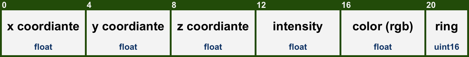
We were able to do some postprocessing on the scan messages that we had already recorded to restructure them into the format that is shown above. There’s actually more information in there (rgb color was added) but the individual point still needs less memory.
As with the color merging described in the following sections, we used the rosbag API to manipulate the rosbag. This removes the need to play the bag and enables the software to process the data faster or slower than realtime (depending on the computer this is run on. Realtime refers to the speed with which the messages were recorded).
3.2 Merge Position and Color
The developed algorithm needs to assign a color to each point in the point cloud. The laser scan message that the lidar device driver generates contains the and coordinate of each point in the coordinate system of the scanner. The position of each point relative to the scanner can be converted to the position of each point relative to some other coordinate system, if we know the transformation (i.e. translation and rotation) between these frames.
The later discussed calibration tool will assist in getting these transformation so it can be seen as given in the development of the coloring algorithm.
The transformation between laser scanner and camera is assumed to be known and given by (can also be computed when the two transforms from robot base to camera and lidar are known). When the lidar returns some point with coordinates , and the transform between lidar and camera can be used to compute the point’s coordinates in the camera’s frame.
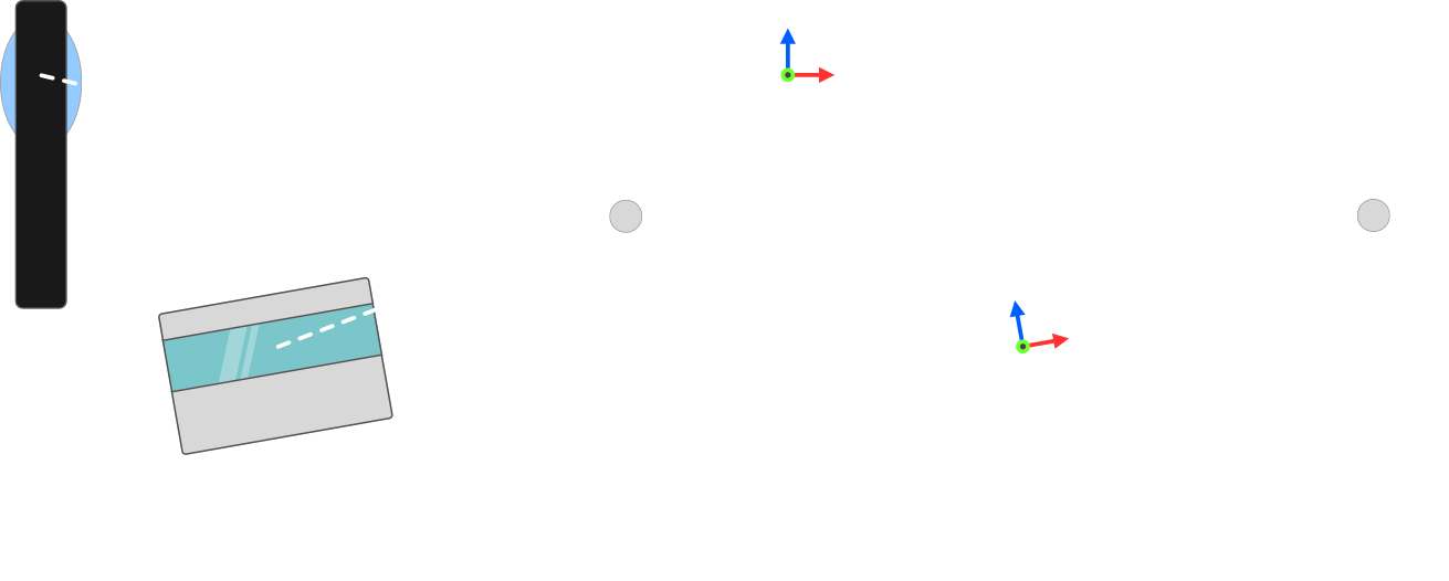
The position of each point will be transformed to a position in the camera’s frame. Since the transformation between lidar and camera does not change, we can use the same transform for each point in a scan message and for every scan message that is captured. After this is done, a mapping from 3D space (, , ) to the 2D image plane (, ) can be applied to get the correct pixel color for each point, as shown in the figure below.
The position of the point is given in cartesian coordinates but can be converted to spherical coordinates. As the length of the resulting vector is not relevant when computing the color mapping, the coordinates , , are converted to angles , .
The image captured by the 360° camera is indexed by pixel positions given as and . The camera does the postprocessing (stitching) of the two lenses automatically and outputs an image that can be wrapped around the camera in the form of a sphere.
Using the angles and , we can compute the pixel coordinates and in the image plane and color the scan points accordingly.
3.3 Implementation Details
The C++ rosbag API is used to access the individual laser scan messages. The API allows to fetch message by message from the bag file. This has several advantages over playing the bag file using rosbag play. The speed of the coloring depends on the processing power of the used computer. Should the processing be faster then realtime (realtime meaning the recording of the messages), the algorithm does not need to wait for the rosbag play node to send new messages. On the other hand, should the computation be slower than realtime, no messages are lost because they could not be computed fast enough.
Cartographer release 1.0 does not have support for colored point cloud messages. Since the message header is dynamic in the way that the fields which describe a point can be ordered in various ways, it can compute a world map from points that have color fields, but it will not add the colors to the output file using the assets writer. This is where the previously discussed fork of the cartographer and its ROS binding cartographer-ros make a difference. The cartographer’s workflow for reading messages from a bag file was altered to also copy the color values to the cartographer’s internal data structure.
3.4 Performance Improvements
The first implementation of the color mapping algorithm got the timestamps for a point cloud message from ROS and then fetched the according video frame using OpenCV. While this method was easy to implement, it was also very slow. Not only would the system only use one CPU core, but it was also throttled by OpenCV having to decode each frame individually.
Modern video encoding mechanisms do not store every frame of the video as a separate image. This would take up far to much memory, even for short movies. Instead, the algorithms will drastically decrease the used memory space by leveraging a very important property of videos: Most of the time, a frame has a lot of similarities with the frames that were recorded shortly before or after it, meaning that frames close to each other in the time domain will likely contain redundant information.
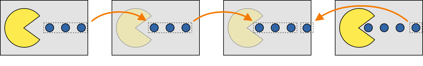
This is why, when videos are encoded, the individual frames are split up into I-, P- and B-frames. An example is shown in the figure above and a quick summary of the different frame type’s properties is given below.
- I-frames contain a whole image.
- P-frames contain information that is stored in frames that were recorded before themselves.
- B-frames can contain information from frames recorded before and after them.
While this technique is useful to minimize memory space needed to store a video, it also comes with a drawback. Decoding a specific image does not only involve one frame, but more likely also other frames that were recorded previously or shortly after. This will slow the decoding down, if frames are decoded out of order. Out of order can mean that only a single frame was skipped, which is rather likely because the camera’s framerate is higher than the scans a lidar records per second.
To prevent this slowdown a video buffer was developed. It will read the video frame by frame (which makes the decoding very fast) and store each frame in its decoded form for at least one second. To further speed up the coloring, the video buffer runs in a separate thread and the code that applies the color to a point cloud is also run in multiple separate threads as shown in the figure below.
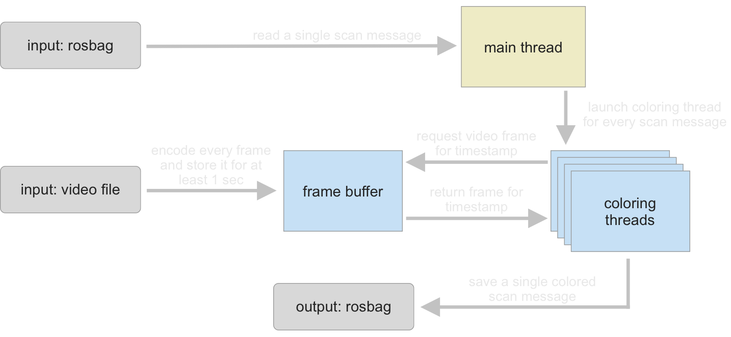
A coloring thread can request a decoded frame and once it’s available, the frame can be used to color the point cloud. Once the coloring is done, the frame is released (deleted from the buffer) and the buffer will continue to fetch new frames from the video file. A frame is deleted after one second if it is not currently in use to color a point cloud. By using this approach, the video decoding can happen way faster (because it is done in chronological order without skipping frames) and each laser scan can still be colored with the correct image frame.
| First Approach | Multithreaded Approach | |
|---|---|---|
| Duration [seconds] | ~288 | ~31 |
The speedup gained by the multithreaded implementation is significant and shown in the table above for a 35 second long video file.
4 Odometry Node
The location of the robot is estimated not only by using the laser scanners but also by using wheel encoders. A wheel encoder counts the revolutions a wheel makes and when summed up over time, can give an estimate of the position of the robot. Wheel odometry is very helpful for small relative position updates but will lead to a huge drift when running for a longer time, meaning that the absolute positioning after a long drive will be far from correct. (Nonetheless, the relative change in position is still useful). The odometry estimate that was used by the robot, was not well tuned. Figure 9 shows the previous odometry estimate (in blue) in comparison to the trajec- tory estimated by the slam algorithm (from laser scanners and blue odometry estimate) and the new odometry estimate (green).
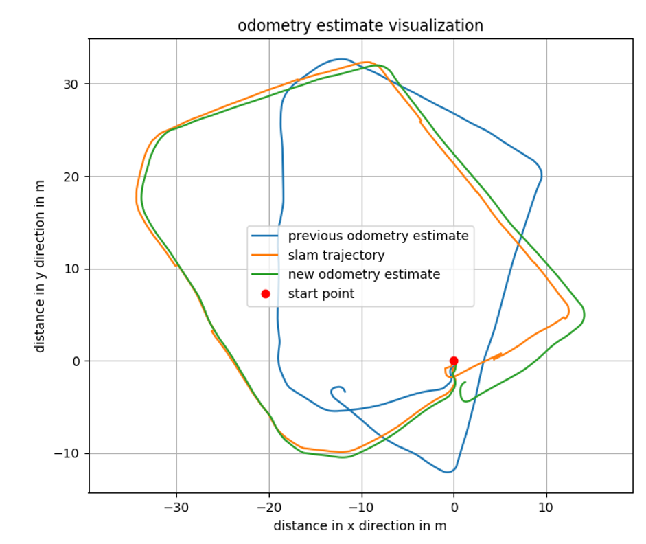
The approach for calculating the odometry estimate was only altered slightly from the one that was already established on the robot when my project partner and I received it. The main difference is the better tuning of the algorithm.
Table 2 shows the estimated offset between the robot’s starting location and the end of its trajectory. (Note that the robot did not start and end at the same position in the real world and the predicted 0.2m offset from the SLAM algorithm seem correct). While the previous odometry estimate has a huge error, the newly parameterized estimate has a very limited error. The estimated trajectory of the SLAM algorithm was used to adjust the odometry node’s parameters.
| SLAM Trajectory | Previous Odometry Estimate | New Estimate | |
|---|---|---|---|
| Position Difference | 0.2m | 12.2m | 2.6m |
We improved the odometry parameterization by running the SLAM algorithm on recorded laser scans. This resulted in a predicted trajectory with decent precision and we used this trajectory to tune the odometry parameters in a way that the trajectory computed from odometry information would closely resemble the path predicted by SLAM.
5 Results