This project is available on GitHub as keypoint-tracking. Every directory has a detailed README.md with useful information.

The work presented here was part of a semester project at the TU Berlin’s Learning & Intelligent Systems Lab.

In the scope of a semester project in university, I worked on augmenting an algorithm for semantic keypoint detection with a LSTM. Keypoints are located on an object and infering the 3D position of multiple keypoints can be used to calculate the pose of the object on which the keypoints are defined. The modification aims to make this system robust, even when keypoints are occluded.

The project is based on work by Lucas Manuelli et al., titled kPam: KeyPoint Affordances for Category-Level Robotic Manipulation. GitHub, Publication

Side note: Due to the pandemic, access to the university’s lab was restricted and all training and testing had to be done in simulation only. I would’ve liked to do the project on a real robot, but this was not possible given the circumstances.

1 Video

Below is a link to the final project video. The first task shows the approach of Manuelli et al. adjusted to the scenario where keypoints are to be detected on the stick. In the second task, one keypoint is occluded and the keypoint detection still works. The last part of the video shows the manipulation pipeline (without occlusion) that will keep pointing the stick’s endpoint to a previously defined location, while the stick’s shape changes.

2 Project Overview

As the project is based on previous work which I was happy to find on GitHub, the first step was adjusting the code to work with the simulation environment. Then some adjustments followed, that made working with a stick possible and at last the network’s architecture was changed to allow processing of time series data.

What follows in this article is an overview over the most important aspects of the project. More detailed information are available in the project report which is linked on GitHub and of course in the commented code.

3 Manipulation Pipeline

The input to the manipulation pipeline is an RGBD image. The keypoint detection algorithm works on an image patch generated from a bounding box around the stick. This makes the first step of the processing pipeline an image segmentation algorithm to find the patch containing the stick. From there, the cropped RGBD image is used as an input to the keypoint detection algorithm. With the 3D positions of each keypoint inferred, the pose of the stick can be estimated. Since the camera’s position is known, the stick’s pose can be translated to world coordinates and manipulation can be performed.

4 Bounding Box Detection

The algorithm used for image segmentation is called maskrcnn-benchmark. It was developed by researchers at facebook, trained for the stick and not further discussed here. Since the algorithm is not longer maintained, I created a fork of the repository and applied changes to keep it usable within the scope of this project.

To not depend on the segmentation for every frame, especially not when a keypoint is occluded, the predicted keypoint pixel positions can be used to generate a bounding box for the next frame.

5 Keypoint Detection Algorithm

The keypoint detection algorithm detects two keypoints on a stick, one at each end. It generates xy pixel positions and a depth estimate in millimeter for each keypoint. Using the camera’s intrinsics, the 3D keypoint positions in camera frame can be calculated.

5.1 Training Data

The data used to train the keypoint detection network shows images of the robot holding the stick. Since the network will be trained to act on time series data, the training data consists of sequences of five images, showing a movement of the stick in the camera’s view. The first image of a sequence is guaranteed to show both keypoints (i.e. endpoints of the stick) without occlusion. The following four images show at least one keypoint, while the other one can be occluded by the robot or some artificially generated geometry.

All training data is generated in the rai simulator and shows sticks with different lengths, varying table and stick colors, and different positions of camera and robot.

The ground truth that is associated with each training image holds each keypoint’s true xy pixel position and depth in millimeter. The data loading scripts used with the project this work is based on, was also used to load the time series data. Before querying batches from the dataset, it was given to a wrapper class that would make sure each sample in a batch consists of five images that show a movement.

Code on GitHub: Loading sequence data

5.2 Loss for symmetric Keypoints

The L1 loss function was used to train the network. In contrary to objects previously used with this algorithm, a stick is symmetric and no clear indexing of keypoints is possible. This required some modifications to the classic L1 loss. Below is the modified loss functions for problems with two symmetric keypoints:

$\text{L1}_\text{symmetrical\_loss} = \min( \mid y_\text{true,1} - y_\text{pred,1} \mid + \mid y_\text{true,2} - y_\text{pred,2} \mid, \mid y_\text{true,1} - y_\text{pred,2} \mid + \mid y_\text{true,2} - y_\text{pred,1} \mid )$

The loss function will try to associate the network’s output with either keypoint and use the minimum of that. This selection process is shown in the leftmost image in the figure below.

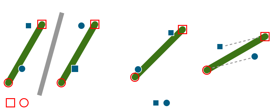
The network is trained on sequences of images because it is supposed to learn to keep track of keypoints even when they are occluded. For these time series data, the loss function decides for the minimum possible loss (given by the equation above) only for the first image of that sequence. All following images in that sequence have to stick to the same mapping. This is done in order to make the network “follow” a keypoint over time and not do the inference solely on data from one frame.

Code on GitHub: Loss function

5.3 Modified Network Structure

The network structure consists of a backbone network and a head network. The backbone network is a ResNet-18 with pre-trained weights. Since the model takes RGBD data as an input, but ResNet is only trained on RGB data, an additional input channel had to be created. The weights of this new input for depth data were initialized by taking the average of the weights of the existing input channels.

The head network uses the output of the ResNet and applies three convolutional layers to it, each followed by batch normalization and a ReLu (rectified linear unit). At the end, another convolutional layer is applied. The output consists of four heatmaps, two for each keypoint to predict a keypoint’s xy-position as well as its depth.

The approach of using heatmaps to detect keypoints is based on work by Sun et al., titled Integral Human Pose Regression. Paper

So far, this is the network architecture used by Manuelli et al. and it is followed by a few additions to make predictions on time series data possible. First, a LSTM is added to the head network. In addition, another stack of convolutional layer, batch normalization, ReLu and convolutional layer are used after the LSTM. This allows the network to keep track of a keypoint’s position, even though it is occluded in the image given to the network.

5.4 Training

At first, the network without LSTM was trained to perform keypoint detection on a stick. The training process for time series data took the learned weights of the previous network as a starting point. This means, that only the LSTM and the few following layers had to be trained. This made training performance on new data pretty good right away from the start.

The network with LSTM was trained with ~80k images showing the stick with domain randomization, on which you can find more details in the section on training data. Five images made up a sequence of images and a batch size of four was used. This means, that the network saw a total of 20 images per batch.

For more information, have a look at the training script.

6 Performance Evaluation

This section discusses the performance of the original network for single image inference and the performance of the modified network with LSTM on time series data. In both cases, the camera that record’s the network’s images is located to the right of the camera that took the images below.

Recordings of the evaluation runs are available on YouTube.

6.1 Single Image Inference

At first, the inference performance of the network developed by Manuelli et al. is evaluated. The training process was adjusted to work on the symmetric stick but other than that, the algorithm is mostly unchanged. The network takes one image as an input, makes a prediction and does not remember any information when performing inference on the next image. Both keypoints where visible to the camera in every frame.

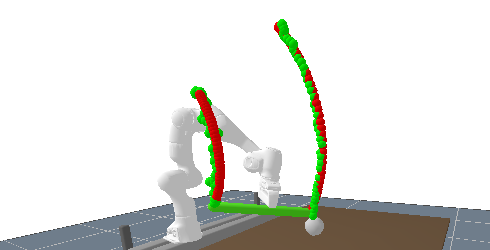
The prediction accuracies of the network are very good and outliers are mostly only present in predictions for the left keypoint, i.e. keypoint 1. This could be caused by the fact that the keypoint was further away from the camera than any example in the training data was.

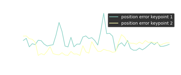
6.2 Time Series Data

The second evaluation step tests the enhanced network with LSTM in a prediction task where one keypoint (keypoint 2) is occluded from frame 18 to 38. For the camera that records the images that are evaluated by the network, this keypoint is hidden behind the wall shown in the right of the image below.

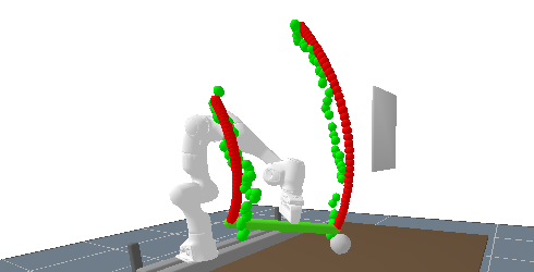
The keypoint prediction is still accurate without occlusion but the error of course grows when one of the keypoints becomes occluded. The prediction accuracy is still good enough to get an estimate for the object’s pose and the prediction accuracy immediately improves when the keypoint comes back into the camera’s view.

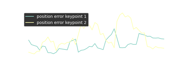
The performance plot above shows the absolute position difference between keypoints for ground truth vs. prediction. When looking into the data in more detail, it becomes clear that even besides the occlusion of a keypoint, the prediction accuracy for xy pixel position is good, but the rising difference between ground truth and prediction originates from inaccuracies in depth prediction.

7 Outlook

The keypoint detection with occlusion shows promising results and I’m very satisfied with the outcome of the project, given that is was only a small semester project in university.

Further improvements could take additional information into account, for example the length of the stick which should not change over the course of the movement. It could be used after first inferring it from an early frame as a prior for inference with occluded keypoints. When one keypoint is visible, the range of possible positions for the other keypoint can be narrowed down.